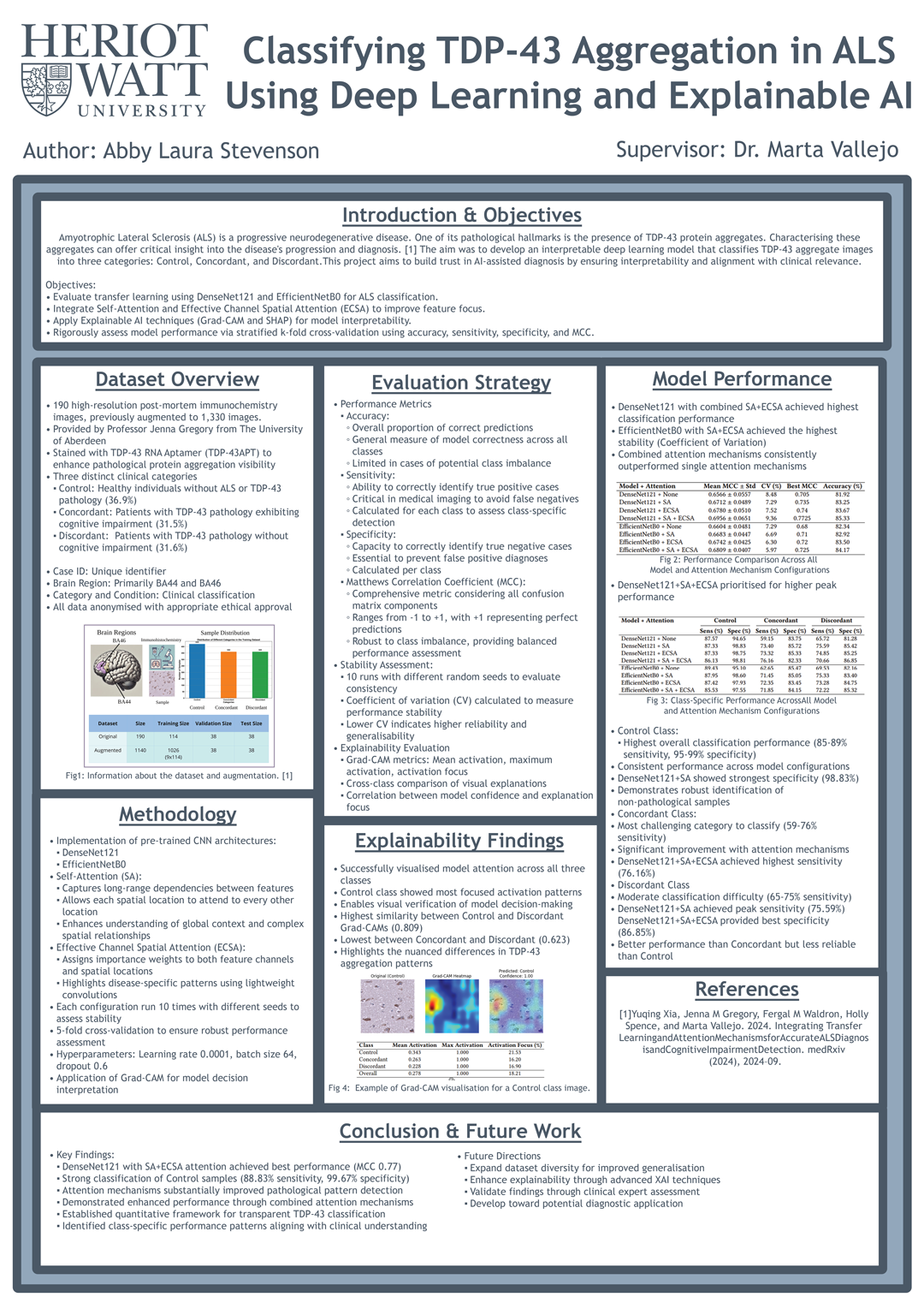
This project was my final-year dissertation, focused on classifying TDP-43 protein aggregation patterns in ALS using deep learning and explainable AI. The aim was to distinguish between three clinical categories: Control (Healthy individuals), Concordant (ALS with cognitive impairment), and Discordant (ALS without cognitive impairment), based on post-mortem immunohistochemistry images.
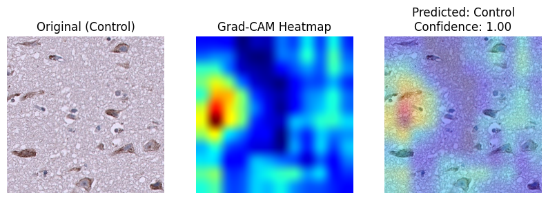
My focus was on evaluating model architectures, attention mechanisms, and explainability techniques to build something trustworthy and informative. I compared DenseNet121 and EfficientNetB0 with combinations of Self-Attention and Effective Channel Spatial Attention (ECSA). The best-performing model (DenseNet121 + SA + ECSA) reached 85.33% accuracy and an MCC of 0.7725. To ensure clinical trust, I used Grad-CAM for explainability and calculated several custom XAI metrics like activation focus and class similarity. The final results show strong performance and reliable interpretability, helping bridge the gap between AI models and clinicians.
Clinicians currently can't distinguish between Concordant and Discordant cases in TDP-43 stained images, which makes this a particularly difficult and important challenge. The goal of this project wasn’t just to classify images, but to help deepen clinical understanding of how ALS presents at the pathological level.
Presenting my research at the Computer Science Poster Day
Develop a deep learning model to accurately classify TDP-43 stained brain tissue into Control, Concordant, and Discordant ALS categories.
Use Grad-CAM to generate transparent and clinically meaningful explanations of the model’s predictions.
Compare DenseNet121 and EfficientNetB0 architectures to identify which works best for this kind of clinical image classification.
Investigate the impact of adding Self-Attention and ECSA modules, both separately and together, to improve feature focus and performance.
I used 190 high-resolution immunohistochemistry images from the University of Aberdeen, this was previously expanded by other researchers to 1,330 through careful, clinically consistent augmentation. These images, stained using a TDP-43 RNA Aptamer, were categorised as Control, Concordant, or Discordant. Proper train/validation/test splits were applied.
I implemented both DenseNet121 and EfficientNetB0 using pre-trained ImageNet weights, then fine-tuned them on the ALS dataset to adapt to domain-specific features. This helped reduce training time while still achieving strong performance.
I added lightweight Self-Attention and Effective Channel Spatial Attention (ECSA) layers to each model variant. Each model was run under four setups: no attention, Self-Attention only, ECSA only, and both combined, to determine which combination best improved model focus.
All models were trained using 5-fold stratified cross-validation with 10 random seeds to ensure stable results. I used the same hyperparameters across experiments: learning rate 0.0001, batch size 64, dropout 0.6, and early stopping to prevent overfitting.
I used Grad-CAM to generate visual explanations for the best-performing model. To go beyond visuals, I also introduced XAI metrics like activation intensity, cross-class similarity, and correlation between confidence and explanation.
# ECSA and Self-Attention blocks
def ECSA_block(input_tensor):
# Channel attention
squeeze = GlobalAveragePooling2D()(input_tensor)
excitation = Dense(units=input_tensor.shape[-1] // 16, activation='relu')(squeeze)
excitation = Dense(units=input_tensor.shape[-1], activation='sigmoid')(excitation)
channel_attention = Multiply()([input_tensor, Reshape((1, 1, input_tensor.shape[-1]))(excitation)])
# Spatial attention
spatial_attention = Conv2D(1, kernel_size=7, padding='same', activation='sigmoid')(channel_attention)
spatial_attention = Multiply()([channel_attention, spatial_attention])
return spatial_attention
def self_attention(input_tensor):
q = Conv2D(filters=input_tensor.shape[-1] // 8, kernel_size=1)(input_tensor)
k = Conv2D(filters=input_tensor.shape[-1] // 8, kernel_size=1)(input_tensor)
v = Conv2D(filters=input_tensor.shape[-1], kernel_size=1)(input_tensor)
attention_scores = tf.matmul(
tf.reshape(q, [tf.shape(q)[0], -1, tf.shape(q)[-1]]),
tf.transpose(tf.reshape(k, [tf.shape(k)[0], -1, tf.shape(k)[-1]]), [0, 2, 1])
)
attention_weights = tf.nn.softmax(attention_scores, axis=-1)
attention_output = tf.matmul(attention_weights,
tf.reshape(v, [tf.shape(v)[0], -1, tf.shape(v)[-1]])
)
attention_output = tf.reshape(attention_output, tf.shape(input_tensor))
return Add()([input_tensor, attention_output])
I implemented lightweight versions of Self-Attention and ECSA attention modules and added them directly to each model's convolutional output. These helped the model learn which features were most relevant for distinguishing between classes while reducing overfitting.
# Evaluate each configuration using 5-fold CV and multiple seeds
def stratified_k_fold_evaluation(X, y, model_builder, k=5, n_seeds=10):
results = []
for seed in range(n_seeds):
np.random.seed(seed)
tf.random.set_seed(seed)
skf = StratifiedKFold(n_splits=k, shuffle=True, random_state=seed)
for train_idx, val_idx in skf.split(X, y):
X_train, X_val = X[train_idx], X[val_idx]
y_train, y_val = y[train_idx], y[val_idx]
model = model_builder()
model.compile(optimizer=Adam(0.0001), loss='categorical_crossentropy', metrics=['accuracy'])
model.fit(X_train, y_train, validation_data=(X_val, y_val), epochs=50, batch_size=64,
callbacks=[EarlyStopping(patience=10, restore_best_weights=True), ReduceLROnPlateau(factor=0.5, patience=5)],
verbose=0)
y_pred = model.predict(X_val)
y_true = np.argmax(y_val, axis=1)
y_pred_classes = np.argmax(y_pred, axis=1)
results.append({
'mcc': matthews_corrcoef(y_true, y_pred_classes),
'accuracy': accuracy_score(y_true, y_pred_classes),
'seed': seed
})
return results
Stratified 5-fold cross-validation was repeated with 10 different seeds to make sure the results were stable and reproducible. All configurations used the same training setup to ensure fair comparison.
# Evaluate overall and per-class performance
def calculate_comprehensive_metrics(y_true, y_pred, class_names):
y_true_classes = np.argmax(y_true, axis=1)
y_pred_classes = np.argmax(y_pred, axis=1)
accuracy = accuracy_score(y_true_classes, y_pred_classes)
mcc = matthews_corrcoef(y_true_classes, y_pred_classes)
sensitivity = recall_score(y_true_classes, y_pred_classes, average=None)
specificity = []
for i in range(len(class_names)):
tn = np.sum((y_true_classes != i) & (y_pred_classes != i))
fp = np.sum((y_true_classes != i) & (y_pred_classes == i))
spec = tn / (tn + fp) if (tn + fp) > 0 else 0
specificity.append(spec)
return {
'accuracy': accuracy,
'mcc': mcc,
'sensitivity': sensitivity,
'specificity': specificity
}
I used both accuracy and Matthews Correlation Coefficient (MCC) to evaluate overall performance, and calculated sensitivity and specificity for each class to understand how well the model recognised each clinical group.
# Compute explainability metrics using Grad-CAM outputs
def calculate_xai_metrics(gradcam_maps, predictions, class_names):
metrics = {}
for i, class_name in enumerate(class_names):
class_maps = [map for j, map in enumerate(gradcam_maps) if np.argmax(predictions[j]) == i]
if class_maps:
metrics[class_name] = {
'mean_activation': np.mean([np.mean(map) for map in class_maps]),
'activation_focus': np.mean([np.sum(map > 0.5) / map.size for map in class_maps]) * 100
}
return metrics
I applied Grad-CAM to the best model (DenseNet121 with ECSA and Self-Attention) and used custom metrics to measure how intense and focused its attention was. This helped make the model's decisions more transparent and clinically meaningful.
Best Configuration: DenseNet121 with both Self-Attention and ECSA performed the strongest overall, reaching a mean MCC of 0.7725 and classification accuracy of 85.33%.
Architecture Comparison: DenseNet121 had the best peak results, but EfficientNetB0 was more consistent across folds, showing lower variation. Both models benefitted from the attention layers, though DenseNet121 handled the pathological complexity better.
Performance comparison across all model and attention mechanism configurations
Control Class: Performed exceptionally well, with a sensitivity of 86.13% and specificity of 98.81%, meaning the model was reliably picking out healthy samples.
Concordant vs Discordant: Concordant cases (ALS with cognitive impairment) were hardest to classify, with sensitivity at 83.23%. Discordant cases (ALS without cognitive impairment) reached 70.66% sensitivity, which is promising given their subtle differences.
Class-specific performance for every DenseNet121 and EfficientNetB0 configuration
Grad-CAM Focus: The Control class had the clearest focus in Grad-CAM maps, with 21.53% of activations concentrated in key regions and a mean activation of 0.343. This suggests the model was picking up clear structural markers in healthy tissue.
Cross-Class Overlap: High similarity (0.809) was found between Control and Discordant attention maps, which could reflect overlapping structural features. Concordant and Discordant samples had the lowest similarity (0.623), pointing to distinct differences in presentation.
Grad-CAM visualisation showing where the model focused to identify protein aggregates in a Control sample
This project marks the end of my undergraduate journey in Computer Science with Artificial Intelligence, and I couldn’t have asked for a more meaningful way to finish. Getting to work with real clinical data from the University of Aberdeen gave me first-hand experience of what it’s like to apply AI to something that actually matters.
Exploring different transfer learning models and attention mechanisms taught me a lot about the importance of good experimental design. Finding that DenseNet121 with both Self-Attention and ECSA gave the best results felt like real proof that the architectural choices I made mattered. It wasn’t just about getting good numbers, it was about building something reliable.
I’ve had the opportunity to present this work a few times now. First at the Machine Learning in Health group meeting at Heriot-Watt, then as part of my final-year Poster Day assessment, and finally at the Women in Data Science 2025 event. I’m currently planning to work with my supervisor, Dr Marta Vallejo, over the summer to develop this project into a publishable research paper. Her support and guidance throughout this project have been invaluable.
Most importantly though, this whole project deepened my understanding and passion for AI in healthcare. I've learned a lot through the course of this project and this has only strengthened my desire to continue pursuing this field.